Crash Course in Relative Entropy I: Mutual Information

The primary input for this discussion is a system \(\Omega\) along with two observables, \(X,Y\):

\[\Omega \overset{(X, Y)}\longrightarrow \mathcal{X}\times\mathcal{Y}\]

These observables allows one to obtain probability distributions on \(\mathcal{X}\times\mathcal{Y}\) from probability distributions on \(\Omega\):

Definition

Pushing forward a probability distribution \(\rho\) on \(\Omega\) gives the marginal distribution:

\[\rho_{X,Y} := (X, Y)_*(\rho) \in \mathrm{Prob}(\mathcal{X}\times\mathcal{Y})\]

This generates two marginal distributions:

\[\begin{split}\rho_X = X_*(\rho) \\ \rho_Y = Y_*(\rho)\end{split}\]

Thse two conditions are insufficient to reconstruct \(\rho_{XY}\) (unless you know that they are independent). This is an amazing feature of probability theory. Without it, probability theory would be quite dull.

Although this is a very abstract definition, it’s an abstraction that effectively encapsulates many useful applications:

Example

Distributions of strings of bits yield enlightening examples. For example, \(X\) could read off the first bit of the string, while \(Y\) reads off the last bit.

In this case \(\rho_X\), is the probability of probability that the first letter in a string is 0/1, while the \(\rho_Y\) is the probability that the last letter in a string is 0/1.

In a general corpus, it is not necessarily the case that:

\[\rho_{XY} \neq \rho_X \cdot \rho_Y\]

As knowledge about the first/last character may carry knowledge of the last/first character.

Entropy & Dependency Between Variables

If \(X\) is independent of \(Y\), the amount of information present in seeing both \(X\) and \(Y\) is the information contained in seeing \(X\) plus the information contained in seeing \(Y\).

At the level of expectation values, we obtain an expression:

\[\mathcal{S}(\rho_{X \times Y}) = \mathcal{S}(\rho_X) + \mathcal{S}(\rho_Y)\]

Warning

We will adopt the standard abusive conflation of random variables and probability distributions, writing the formula below as:

\[\mathcal{S}(X,Y) = \mathcal{S}(X) + \mathcal{S}(Y)\]

We’d like to emphasize that the left side is the entropy of a joint distribution, while the right side is a sum of entropies of marginal distributions.

Note

Somewhat surprising, this additivity characterizes independence.

In general, this formula may “overestimate” the entropy:

\[\mathcal{S}(X, Y) \leq \mathcal{S}(X) + \mathcal{S}(Y)\]

In other words, dependence between variables decreases entropy. Therefore, the amount of this decrease can therefore be considered as a metric for how much \(X\) and \(Y\) depend on each other.

Mutual Information

Definition

The mutual information between \(X\) and \(Y\) is defined as:

\[I(X, Y) = \mathcal{S}(X) + \mathcal{S}(Y) - \mathcal{S}(X,Y) \in \mathbb{R}\]

Note

If X and Y were independent, the sum of the first two terms is the entropy of \(X\) and \(Y\). Therefore, the mutual information is how much you overestimated the average amount of information, were you to assume they were independent.

Note

As entropy is invariant under symmetries, mutual information is “symmetric.”

There is another formulation: mutual information is just the entropy of \(X\) minus the average amount of information in \(X\) when \(Y\) is known. This formulation relies upon a common “forgetful” Bayesian contrustion:

\[\mathrm{Prob}(X \times Y) \longrightarrow \mathrm{Maps}(X, \mathrm{Prob}(Y))\]

In other words, we assemble a joint distribution conditioned on observations of \(X\) into a map associating an event \(x \in X\) to the probability distribtion on \(Y\):

\[\rho_{X, Y}|_{x} = \rho_{X,Y}( - | x )\]

conventionally referred to as the conditional distribution.

Taking the entropy of this distribution conditional distribution gives a function whose expectation value is intimately related to mutual information:

Note

\[I(X, Y) = \mathcal{S}(X , Y) - \langle \mathcal{S}(\rho_{X, Y}|_{x}) \rangle_{\rho_X}\]

Example: Noisy Channel

In signal processing, mutual information quantifies to what extent one system is the signal/receiver for another.

Example

\(X\) could be the presence of a certain type of stimuli, and \(Y\) could be the activation of a neuron some time later.

In this case, a low amount of mutual information refutes the hypothesis that \(X\) can be considered as a stimuli for \(Y\).

Let’s imagine the stimuli \(X\) and the neuron \(Y\) can only take two states \(x_0, x_1\) and \(y_0, y_1\). Moreover, let’s for simplicity, let’s assume that:

\[P(y_0 | x_0) = P(y_1 | x_1) = p\]

As we have control over the stimuli, let’s assume that:

\[P(x_0) = P(x_1) = \frac{1}{2}\]

(i.e. for simplicity assume it’s in a maximally entropic state). This can be visualized as a weighted bipartitie graph:

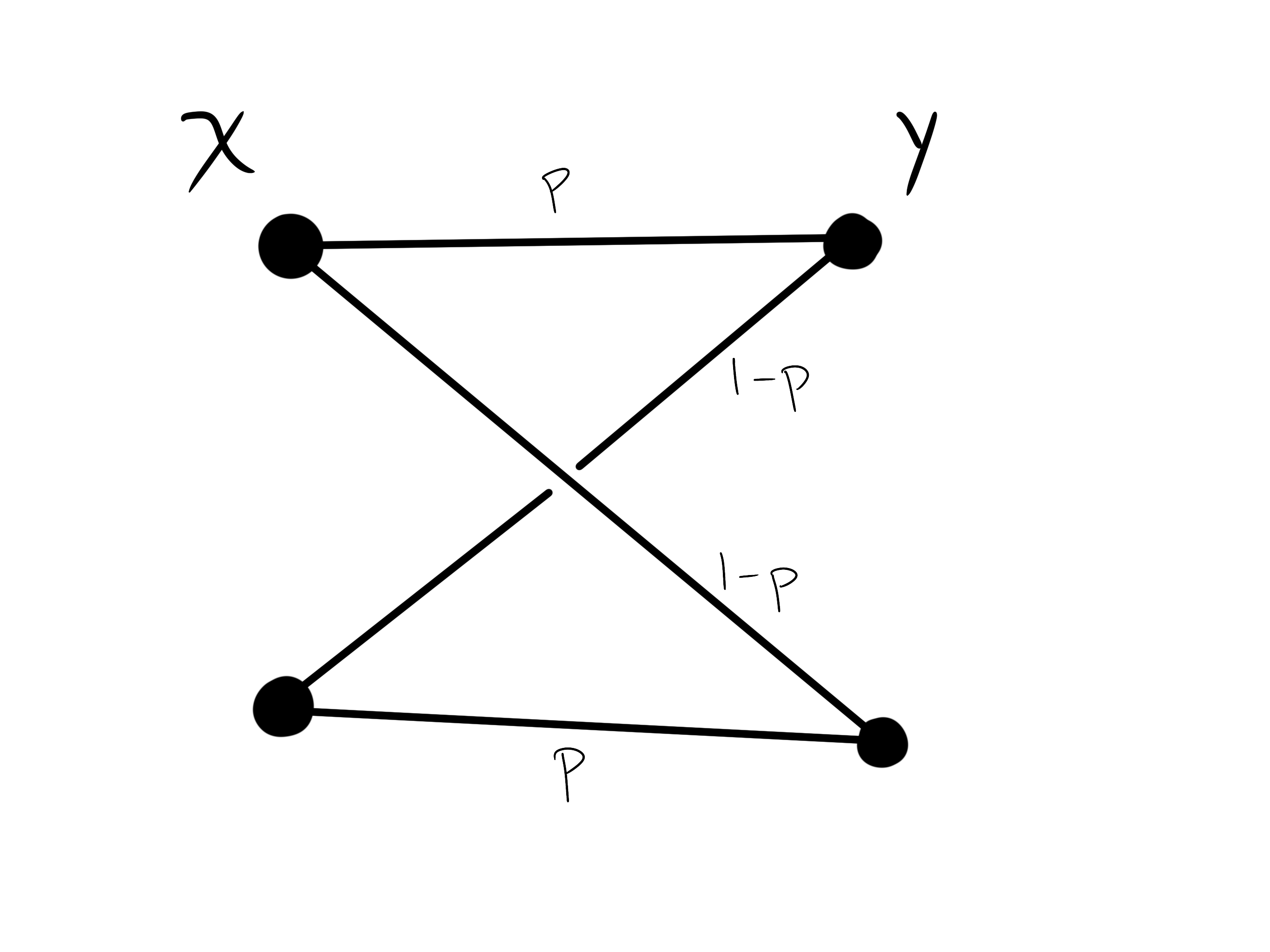
Therefore, the mutual information is a function of a single variable \(p\), which we can think of as the “strength of the signal.”

Note

When \(p \neq 1\), the channel is “noisy.”

With some work, one can show:

\[I(X, Y) = 1 - \mathcal{S}(p, 1-p)\]

As the second term is the entropy in \(Y\) (the response) when \(X\) (the stimuli) is known.

Note

The mutual information is minimized when the channel is the noisiest, and is maximized when it is pristine: \(p = 0\) or \(p = 1\) (in which case it is 1).

These are the case because the former case maximizes entropy, while the latter maximizes entropy of the marginal distribution \(\rho_Y\).

More generally, there is some one-to-one correspondence between \(X\) and \(Y\):

\[\frac{I(X, Y)}{\sqrt{\mathcal{S}(X)\mathcal{S}(Y)}} = 1\]

Indicating that they are in some sense “perfectly correlated” (the one-to-one correspondence is \(x_i \leftrightarrow y_i\) when \(p = 1\)).

Note

This quantity may be thought of as analogous to a Pearson correlation coefficient. However, while the mutual information merely indicates the strength of a relationship, correlations say something about the form of the relationship.

Example: Correlated Gaussians

Let’s say we’re considering a 2D gaussian with features \(X\) and \(Y\), Pearson correlation coefficient \(c_{XY}\), and equal standard deviations. In this case, the mutual information takes on an elegant form:

\[I(X, Y) = -\frac{1}{2} \log (1 - c_{XY}^2)\]

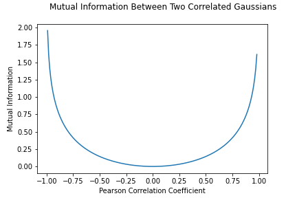
In other words:

• “perfectly correlated” Gaussian features have infinite mutual information!

• independent features have no mutual information.

Note

This gives a conceptual, heuristic interpretation of Principal Component Analysis: you’re finding composite features which contain no information about each other.

Mutual information is about comparing two distributions: the “real” distribution and the distribution which assume the features are independent. In other words, mutual information is a “relative” notion of entropy.